HOMEWORK PART I
Question #1
Write code to return the percentage of people who were frisked for each race. In other words, count up the number of people who were frisked for a given race divided by the number of people of that race stopped. Which race leads to the highest percentage of frisks? Which one the lowest?
The race leading to the highest percentage of frisks is Black Hispanic at 59.7%
The race leading to the lowest percentage of frisks is White at 41.9%.
Question #2
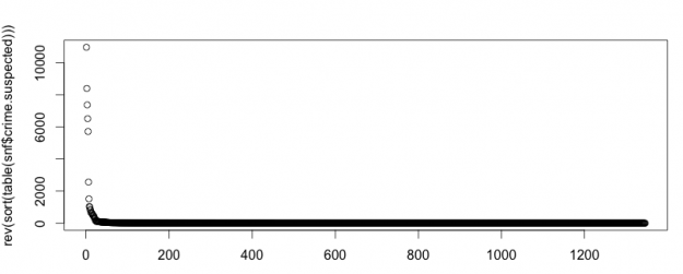
Plot the number of times each crime occurs in descending order (we’ve learned a couple of ways to do this, though using sort(), table() and that new type= parameter to plot() is your best bet). What does this distribution of crimes look like? In other words, are there an equal number of every kind of crime or are there a few that dominate?
No, they are not equally distributed. There are a few that make up most of the crimes suspected.

Question #3
Well I’m kind of answering that question for you here – let’s take the top 30 suspected crimes and look at those. If we were to just look at stops where the crime.suspected was one of the top 30 crimes, what percentage of the stops would that cover? Do you think that’s enough?
The top 30 crimes suspected cover 91.3% of all crimes suspected. I think that that would be enough.
Question #4
Write code to create a variable called “crime.abbv” that consists of just the first three letters of crime.suspected and show the code to add it to our main data frame. Now what percentage of the stops do the top 30 crime.abbvs account for?
Now, using the abbreviated names for the crimes suspected, the top 30 make up 98.4% of all crimes.
HOMEWORK PART II

